Kiva Project#

(adapted from https://bit.ly/2J7G9f8)

PROBLEM:#

Context#

Kiva.org is an online crowdfunding platform to extend financial services to poor and financially excluded people around the world. Kiva lenders have provided over $1 billion dollars in loans to over 2 million people.

In order to set investment priorities, help inform lenders, and understand their target communities, knowing the level of poverty of each borrower is critical. However, this requires inference based on a limited set of information for each borrower.

Submissions in this challenge will take the form of Python data analysis.

Kiva has provided a dataset of loans issued over the 2014-2018 time period, and participants are invited to use this data as well as source external public datasets to help Kiva build models for assessing borrower welfare levels. With a stronger understanding of their borrowers and their poverty levels, Kiva will be able to better assess and maximize the impact of their work.

Problem statement#

For the locations in which Kiva has active loans, the objective is to pair Kiva’s data with additional data sources to estimate the welfare level of borrowers in specific regions, based on shared economic and demographic characteristics.

A good solution would connect the features of each loan or product to one of several poverty mapping datasets, which indicate the average level of welfare in a region on as granular a level as possible. Many datasets indicate the poverty rate in a given area, with varying levels of granularity. Kiva would like to be able to disaggregate these regional averages by gender, sector, or borrowing behavior in order to estimate a Kiva borrower’s level of welfare using all of the relevant information about them. Strong submissions will attempt to map vaguely described locations to more accurate geocodes.

Personal disclaimer#

From a research perspective, the results obtained are never going to be a full representation of the realities that borrowers experience. It is meant to spark a discussion around how we can identify the welfare level of borrowers and improve them where we can.

SOLUTION:#

Python Packages & Functions#

Here we upload all the Python packages and datasets required for analysis.

# Packages
import numpy as np

import pandas as pd

import matplotlib.pyplot as plt
import matplotlib.dates as mdates

Data#

1. Original Data#

loan_data = pd.read_csv('C://Users//CT//Documents//GitHub//knowledge-hub//book//data//kiva-project//kiva_loans.csv')

location_data = pd.read_csv('C://Users//CT//Documents//GitHub//knowledge-hub//book//data//kiva-project//kiva_mpi_region_locations.csv')

loan_themes  = pd.read_csv('C://Users//CT//Documents//GitHub//knowledge-hub//book//data//kiva-project//loan_theme_ids.csv')

regional_lts = pd.read_csv('C://Users//CT//Documents//GitHub//knowledge-hub//book//data//kiva-project//loan_themes_by_region.csv')

dfs = {'loan_data':loan_data, 'location_data':location_data,
       'loan_themes':loan_themes, 'regional_lts':regional_lts}

for key, val in dfs.items():

    print(str(key+' shape:'), val.shape)

loan_data shape: (671205, 20)
location_data shape: (2772, 9)
loan_themes shape: (779092, 4)
regional_lts shape: (15736, 21)

Descriptions of the original datasets

There are four data sources provided by Kiva:

loan_data
1. id - Unique ID for loan
2. funded_amount - The amount disbursed by Kiva to the field agent (USD)
3. loan_amount - The amount disbursed by the field agent to the borrower (USD)
4. activity - More granular category
5. sector - High level category
6. use - Exact usage of loan amount
7. country_code - ISO country code of country in which loan was disbursed
8. country - Full country name of country in which loan was disbursed
9. region - Full region name within the country
10. currency - The currency in which the loan was disbursed
11. partner_id - ID of partner organization
12. posted_time - The time at which the loan is posted on Kiva by the field agent
13. disbursed_time - The time at which the loan is disbursed by the field agent to the borrower
14. funded_time - The time at which the loan posted to Kiva gets funded by lenders completely
15. term_in_months - The duration for which the loan was disbursed in months
16. lender_count - The total number of lenders that contributed to this loan
17. tags
18. borrower_genders - Comma separated M,F letters, where each instance represents a single male/female in the group
19. repayment_interval
20. date

location_data
1. LocationName - region, country
2. ISO - some sort of unique abbreviation for country
3. country - country
4. region - region within country
5. world_region - parts of the world
6. MPI - multidimensional poverty index
7. geo - (latitude, longitude)
8. lat - latitude
9. lon - longitude

loan_themes
1. id - Unique ID for loan (Loan ID)
2. Loan Theme ID - ID for Loan Theme
3. Loan Theme Type - Category name of type of loan
4. Partner ID

regional_lts
1. Partner ID
2. Field Partner Name
3. sector
4. Loan Theme ID
5. Loan Theme Type
6. country
7. forkiva
8. region
9. geocode_old
10. ISO
11. number
12. amount
13. LocationName
14. geocode
15. names
16. geo
17. lat
18. lon
19. mpi_region
20. mpi_geo
21. rural_pct

2. Supplementary Data#

In this section, we aim to gather the following data from the World Bank:

Per Capita Expenditure (PCE) for each country - this is the total market value of all purchases in a country divided by that country’s total population (data: https://bit.ly/3blw0be)

# Per Capita Expenditure
PCE_data = pd.read_csv('C://Users//CT//Documents//GitHub//knowledge-hub//book//data//kiva-project//PCE data.tsv', sep='\t')

print('PCE data shape:',PCE_data.shape)

PCE_data = PCE_data.drop(['Unnamed: 61'],axis=1) # dropping the column containing only NaN values

PCE data shape: (185, 62)

# add this dataset to the dictionary
dfs['PCE_data'] = PCE_data

dfs.keys()

dict_keys(['loan_data', 'location_data', 'loan_themes', 'regional_lts', 'PCE_data'])

Data Summary#

for key, val in dfs.items():

    # 1. Get the summary table
    num_summary = val.describe()
    cat_summary = val.loc[:,val.dtypes==np.object].describe(include=['O'])
    
    # 2. Display it

    print('\nSUMMARY STATISTICS WITHOUT AGGREGATION: {}'.format(key),'\n')
    
    display(num_summary)
    
    print('\n')
    
    display(cat_summary)
    
    print('\n')

SUMMARY STATISTICS WITHOUT AGGREGATION: loan_data

	id	funded_amount	loan_amount	partner_id	term_in_months	lender_count
count	6.712050e+05	671205.000000	671205.000000	657698.000000	671205.000000	671205.000000
mean	9.932486e+05	785.995061	842.397107	178.199616	13.739022	20.590922
std	1.966113e+05	1130.398941	1198.660073	94.247581	8.598919	28.459551
min	6.530470e+05	0.000000	25.000000	9.000000	1.000000	0.000000
25%	8.230720e+05	250.000000	275.000000	126.000000	8.000000	7.000000
50%	9.927800e+05	450.000000	500.000000	145.000000	13.000000	13.000000
75%	1.163653e+06	900.000000	1000.000000	204.000000	14.000000	24.000000
max	1.340339e+06	100000.000000	100000.000000	536.000000	158.000000	2986.000000

	activity	sector	use	country_code	country	region	currency	posted_time	disbursed_time	funded_time	tags	borrower_genders	repayment_interval	date
count	671205	671205	666973	671197	671205	614405	671205	671205	668809	622874	499789	666984	671205	671205
unique	163	15	424912	86	87	12695	67	667399	5719	498007	86719	11298	4	1298
top	Farming	Agriculture	to buy a water filter to provide safe drinking...	PH	Philippines	Kaduna	PHP	2017-05-15 00:00:00+00:00	2017-02-01 08:00:00+00:00	2016-09-21 13:03:24+00:00	user_favorite	female	monthly	2017-03-20
freq	72955	180302	5217	160441	160441	10000	160440	25	2800	33	27088	426502	342717	1308

SUMMARY STATISTICS WITHOUT AGGREGATION: location_data

	MPI	lat	lon
count	984.000000	892.000000	892.000000
mean	0.211330	9.169710	16.635888
std	0.183621	16.484531	61.234566
min	0.000000	-34.947896	-122.747131
25%	0.053000	-1.027901	-12.819854
50%	0.155000	11.211379	26.419389
75%	0.341500	18.084292	47.019436
max	0.744000	49.264748	138.581284

	LocationName	ISO	country	region	world_region	geo
count	984	1008	1008	984	1008	2772
unique	984	102	102	928	6	881
top	Badakhshan, Afghanistan	NGA	Nigeria	Central	Sub-Saharan Africa	(1000.0, 1000.0)
freq	1	37	37	8	432	1880

SUMMARY STATISTICS WITHOUT AGGREGATION: loan_themes

	id	Partner ID
count	7.790920e+05	764279.000000
mean	1.047475e+06	180.825840
std	2.282538e+05	97.914029
min	6.386310e+05	9.000000
25%	8.499768e+05	126.000000
50%	1.046528e+06	145.000000
75%	1.244768e+06	204.000000
max	1.444243e+06	557.000000

	Loan Theme ID	Loan Theme Type
count	764279	764279
unique	956	203
top	a1050000000wf0q	General
freq	110264	380693

SUMMARY STATISTICS WITHOUT AGGREGATION: regional_lts

	Partner ID	number	amount	lat	lon	rural_pct
count	15736.000000	15736.000000	1.573600e+04	13662.000000	13662.000000	14344.000000
mean	191.376144	53.628432	2.003991e+04	14.328878	29.433569	68.084635
std	118.705003	403.079799	9.636941e+04	16.757689	83.255739	26.550064
min	9.000000	1.000000	2.500000e+01	-34.610548	-172.790661	0.000000
25%	123.000000	1.000000	9.500000e+02	6.266728	-71.967463	60.000000
50%	154.000000	4.000000	2.600000e+03	13.484101	41.899993	73.000000
75%	217.000000	15.000000	8.750000e+03	22.189940	106.677321	85.000000
max	545.000000	22538.000000	4.929900e+06	51.314017	159.972900	100.000000

	Field Partner Name	sector	Loan Theme ID	Loan Theme Type	country	forkiva	region	geocode_old	ISO	LocationName	geocode	names	geo	mpi_region	mpi_geo
count	15736	15736	15736	15736	15736	15736	15736	1200	15722	15736	13662	13661	15736	15722	9671
unique	302	11	718	170	79	2	9526	340	77	9561	6557	6275	6558	392	335
top	Alalay sa Kaunlaran (ASKI)	General Financial Inclusion	a1050000000wf0V	General	Philippines	No	Chouf	(-1.2833333, 36.8166667)	PHL	Chouf, Lebanon	[(19.7126764, 105.8393447)]	Philippines	(1000.0, 1000.0)	Northern Mindanao, Philippines	(8.020163499999999, 124.6856509)
freq	1207	13679	1152	5661	3467	13211	25	20	3467	25	43	137	2074	1174	1174

SUMMARY STATISTICS WITHOUT AGGREGATION: PCE_data

	Country	1960	1961	1962	1963	1964	1965	1966	1967	1968	...	2010	2011	2012	2013	2014	2015	2016	2017	2018	2019
count	185	43	44	45	45	47	50	51	52	52	...	178	164	163	162	160	158	157	156	152	137
unique	185	43	44	45	45	47	50	51	52	52	...	178	164	163	162	160	158	157	156	152	137
top	East Asia and Pacific	358.28	376.28	391.98	366.59	359.69	358.46	343.77	364.11	386.75	...	7,168.46	6,887.91	6,766.62	6,988.29	7,035.26	7,013.70	7,098.35	7,113.80	7,152.70	923.25
freq	1	1	1	1	1	1	1	1	1	1	...	1	1	1	1	1	1	1	1	1	1

4 rows × 61 columns

	Country	1960	1961	1962	1963	1964	1965	1966	1967	1968	...	2010	2011	2012	2013	2014	2015	2016	2017	2018	2019
count	185	43	44	45	45	47	50	51	52	52	...	178	164	163	162	160	158	157	156	152	137
unique	185	43	44	45	45	47	50	51	52	52	...	178	164	163	162	160	158	157	156	152	137
top	East Asia and Pacific	358.28	376.28	391.98	366.59	359.69	358.46	343.77	364.11	386.75	...	7,168.46	6,887.91	6,766.62	6,988.29	7,035.26	7,013.70	7,098.35	7,113.80	7,152.70	923.25
freq	1	1	1	1	1	1	1	1	1	1	...	1	1	1	1	1	1	1	1	1	1

4 rows × 61 columns

Exploratory Data Analysis#

The impact of KIVA donors#

In this section, we seek to explore the data to answer certain questions around KIVA donor contributions.

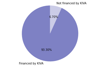
1. How much of the total loan amount has Kiva financed?

# 1. Calculate the percentage of loan requests that have been funded
percentage1 = (loan_data.funded_amount.sum()/loan_data.loan_amount.sum())*100
percentage1 = round(percentage1, 2)

# 2. Display the result
status = ['Financed by KIVA','Not financed by KIVA']

values = [percentage1, (100-percentage1)]

fig1, ax1 = plt.subplots()

ax1.pie(values, labels=status,
        autopct='%1.2f%%',
        startangle=90,
        colors=np.array(['#7e81c4','#cbcce7']))

ax1.axis('equal')  # Equal aspect ratio ensures that pie is drawn as a circle.

plt.show()

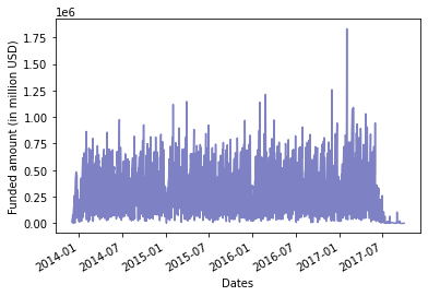
2. How much money have Kiva donors contributed over time?

print('\n', 'DAILY CONTRIBUTIONS OF KIVA DONORS AS A COLLECTIVE')

# convert datetime values to appropriate formats
loan_data['posted_time'] = loan_data['posted_time'].astype('datetime64')
loan_data['disbursed_time'] = loan_data['disbursed_time'].astype('datetime64')
loan_data['funded_time'] = loan_data['funded_time'].astype('datetime64')

# pick out dates
loan_data.loc[:,'disbursement_date'] = loan_data['disbursed_time'].dt.date

# create a pivot-table
tab1 = pd.pivot_table(loan_data, values='funded_amount', index=['disbursement_date'], aggfunc='sum')

# plot this table
from pandas.plotting import register_matplotlib_converters
register_matplotlib_converters()

fig, ax = plt.subplots()

ax.plot(tab1.index, tab1['funded_amount'], color='#7e81c4')

# rotate and align the tick labels so they look better
fig.autofmt_xdate()

# declare the title and show the completed graph

plt.xlabel('Dates')

plt.ylabel('Funded amount (in million USD)')

plt.show()

 DAILY CONTRIBUTIONS OF KIVA DONORS AS A COLLECTIVE

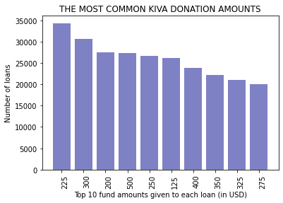
3. How much money have Kiva donors given to individual loans?

# create a pivot-table
loan_count_per_funded_amount = pd.pivot_table(loan_data, values='id', index=['funded_amount'], aggfunc='count')

# rename the column
loan_count_per_funded_amount.columns = ['number_of_loans']

# sort the results in descending order
loan_count_per_funded_amount = loan_count_per_funded_amount.sort_values(by=['number_of_loans'], ascending=False)

# and display top 10 results
amounts = ['225','300','200','500','250','125','400','350','325','275']

fig, ax = plt.subplots()

ax.bar(amounts,loan_count_per_funded_amount.iloc[0:10,0],color='#7e81c4')

plt.ylabel('Number of loans')

ax.set_xticklabels(labels=amounts, rotation = (90), fontsize = 10, va='top', ha='left')

plt.xlabel('Top 10 fund amounts given to each loan (in USD)')

plt.title('THE MOST COMMON KIVA DONATION AMOUNTS')

plt.show()

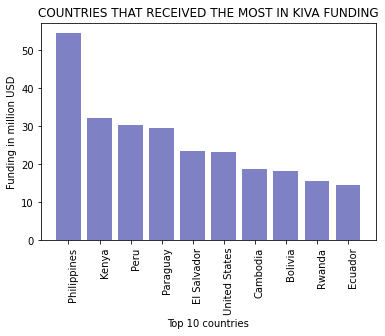
4. How much money have Kiva donors given to individual countries?

# create a pivot-table
tab2 = pd.pivot_table(loan_data, values='funded_amount', index=['country'], aggfunc='sum')

# sort the results in descending order
tab2 = tab2.sort_values(by=['funded_amount'], ascending=False)

# rename the aggregated column to an appropiate label
tab2.columns = ['sum_of_funded_amount']

# make some index entries into columns
tab2 = tab2.reset_index(level=['country'])

# and display top 10 results

fig, ax = plt.subplots()

ax.bar(tab2.iloc[0:10,0],(tab2.iloc[0:10,1]/1000000),color='#7e81c4')

plt.ylabel('Funding in million USD')

ax.set_xticklabels(labels=tab2.iloc[0:10,0], rotation = (90), fontsize = 10, va='top', ha='left')

plt.xlabel('Top 10 countries')

plt.title('COUNTRIES THAT RECEIVED THE MOST IN KIVA FUNDING')

plt.show()

# create a pivot-table
loans_per_country = pd.pivot_table(loan_data, values='id', index=['country'], aggfunc='count')

# sort the results in descending order
loans_per_country = loans_per_country.sort_values(by=['id'], ascending=False)

# rename the aggregated column to an appropiate label
loans_per_country.columns = ['number_of_loans']

# make some index entries into columns
loans_per_country = loans_per_country.reset_index(level=['country'])

# and display top 10 results
loans_per_country.head(10)

# and display top 10 results

fig, ax = plt.subplots()

ax.bar(loans_per_country.iloc[0:10,0],loans_per_country.iloc[0:10,1],color='#7e81c4')

plt.ylabel('Number of loans')

ax.set_xticklabels(labels=tab2.iloc[0:10,0], rotation = (90), fontsize = 10, va='top', ha='left')

plt.xlabel('Top 10 countries')

plt.title('COUNTRIES THAT HAD THE HIGHEST NUMBER OF LOANS ON KIVA')

plt.show()

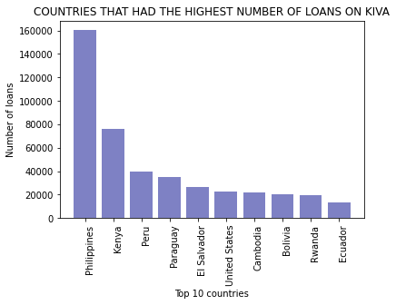
This shows that the top 10 countries in terms of the number of loans and amount of funding from KIVA were the same and each country maintained its position.

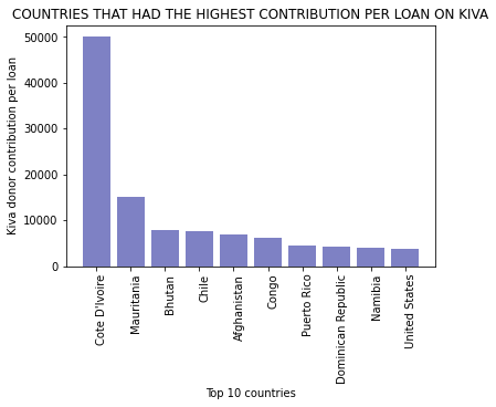
Countries that had the highest contribution per loan were:

# initial status message
print('The shape of tab2 before merge: ', tab2.shape)

# join the data, keeping only relevant entries
tab2 = tab2.merge(loans_per_country, on='country')

# final status message
print('The shape of tab2 after merge: ', tab2.shape)

The shape of tab2 before merge:  (87, 2)
The shape of tab2 after merge:  (87, 3)

# add a calculated column to the newly merged tab2
tab2.loc[:, 'contribution_per_loan'] = tab2['sum_of_funded_amount']/tab2['number_of_loans']

# sort the results in descending order
tab2 = tab2.sort_values(by=['contribution_per_loan'], ascending=False)

# and display top 10 results

fig, ax = plt.subplots()

ax.bar(tab2.iloc[0:10,0], round(tab2.iloc[0:10,3], 2), color='#7e81c4')

plt.ylabel('Kiva donor contribution per loan')

ax.set_xticklabels(labels=tab2.iloc[0:10,0], rotation = (90), fontsize = 10, va='top', ha='left')

plt.xlabel('Top 10 countries')

plt.title('COUNTRIES THAT HAD THE HIGHEST CONTRIBUTION PER LOAN ON KIVA')

plt.show()

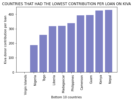
Countries that had the lowest contribution per loan were:

# add a calculated column to the newly merged tab2
tab2.loc[:, 'contribution_per_loan'] = tab2['sum_of_funded_amount']/tab2['number_of_loans']

# sort the results in ascending order
tab2 = tab2.sort_values(by=['contribution_per_loan'], ascending=True)

# and display top 10 results

fig, ax = plt.subplots()

ax.bar(tab2.iloc[0:10,0], round(tab2.iloc[0:10,3], 2), color='#7e81c4')

plt.ylabel('Kiva donor contribution per loan')

ax.set_xticklabels(labels=tab2.iloc[0:10,0], rotation = (90), fontsize = 10, va='top', ha='left')

plt.xlabel('Bottom 10 countries')

plt.title('COUNTRIES THAT HAD THE LOWEST CONTRIBUTION PER LOAN ON KIVA')

plt.show()

5. What is the geographical footprint of where funds given by KIVA donors end up?

# make a copy of the loan_data dataset and combine it with partner data
loan_data_copy = loan_data.copy()

# ensure that the common column is the same datatype and they share the same name
# the datatype chosen was float64 to preserve any decimal points
print(loan_data_copy.iloc[:,10].name) # original name; stays the same
print('')

print(regional_lts.iloc[:,0].name) #original name - will be changed
#change column name
regional_lts.columns = ['partner_id', 'Field Partner Name', 'sector',
                        'Loan Theme ID', 'Loan Theme Type', 'country',
                        'forkiva', 'region', 'geocode_old',
                        'ISO', 'number', 'amount',
                        'LocationName', 'geocode', 'names',
                        'geo', 'lat', 'lon',
                        'mpi_region', 'mpi_geo', 'rural_pct']
# confirm change
print(regional_lts.iloc[:,0].name)

# change the datatype
regional_lts.iloc[:,0] = regional_lts.iloc[:,0].astype('float64')

partner_id

Partner ID
partner_id

# create a pivot-table
tab3 = pd.pivot_table(loan_data_copy, values='funded_amount', index=['partner_id'], aggfunc='sum')

# sort the results in descending order
tab3 = tab3.sort_values(by=['funded_amount'], ascending=False)

# rename the aggregated column to an appropiate label
tab3.columns = ['sum_of_funded_amount']

# make some index entries into columns
tab3 = tab3.reset_index(level=['partner_id'])

# create another pivot-table
tab4 = pd.pivot_table(regional_lts, values='amount',
                      index=['partner_id', 'Field Partner Name',
                             'country'],
                      aggfunc='count')

# sort the results in descending order
tab4 = tab4.sort_values(by=['amount'], ascending=False)

# rename the aggregated column to an appropiate label
tab4.columns = ['count_of_amount']

# make some index entries into columns
tab4 = tab4.reset_index(level=['partner_id', 'Field Partner Name', 'country'])

# create a third pivot-table
tab5 = pd.pivot_table(loan_data_copy, values='id', index=['partner_id'], aggfunc='count')

# sort the results in descending order
tab5 = tab5.sort_values(by=['id'], ascending=False)

# rename the aggregated column to an appropiate label
tab5.columns = ['number_of_loans']

# make some index entries into columns
tab5 = tab5.reset_index(level=['partner_id'])

# initial status message
print('The shape of tab3 before merge: ', tab3.shape)

# join the data, keeping only relevant entries
tab3 = tab3.merge(tab5, on='partner_id')

# final status message
print('The shape of tab3 after merge: ', tab3.shape)


# initial status message
print('The shape of tab3 before merge: ', tab3.shape)

# join the data, keeping only relevant entries
tab3 = tab3.merge(tab4, on='partner_id')

# final status message
print('The shape of tab3 after merge: ', tab3.shape)


percentage2 = tab3.shape[0]/366 * 100
percentage2 = round(percentage2, 0)

print('Out of the 366 partners that disbursed loans, KIVA had the contact details of '+str(percentage2)+'% of them.')

The shape of tab3 before merge:  (366, 2)
The shape of tab3 after merge:  (366, 3)
The shape of tab3 before merge:  (366, 3)
The shape of tab3 after merge:  (331, 6)
Out of the 366 partners that disbursed loans, KIVA had the contact details of 90.0% of them.

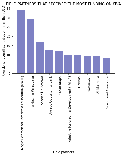
The partners that received the most funding by KIVA were:

# to have more details of the partners that received the most funding by KIVA,
# sort the results in descending order
tab3 = tab3.sort_values(by=['sum_of_funded_amount'], ascending=False)

# drop the unecessary columns
tab3 = tab3.drop('count_of_amount',1)

# display top 10 results; do they match with the original tab3? They match!

fig, ax = plt.subplots()

ax.bar(tab3.iloc[0:10,3], (tab3.iloc[0:10,1]/1000000), color='#7e81c4')

plt.ylabel('Kiva donor overall contribution (in million USD)')

ax.set_xticklabels(labels=tab3.iloc[0:10,3], rotation = (90), fontsize = 10, va='top', ha='left')

plt.xlabel('Field partners')

plt.title('FIELD PARTNERS THAT RECEIVED THE MOST FUNDING ON KIVA')

plt.show()

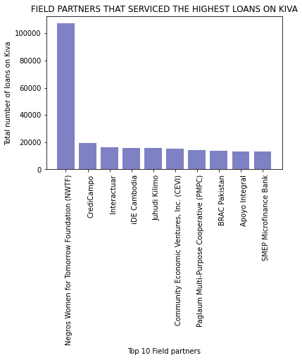
The partners that serviced the highest number of loans on KIVA were:

# sort the results in descending order
tab3 = tab3.sort_values(by=['number_of_loans'], ascending=False)

# display top 10 results in terms of number of loans

fig, ax = plt.subplots()

ax.bar(tab3.iloc[0:10,3], tab3.iloc[0:10,2], color='#7e81c4')

plt.ylabel('Total number of loans on Kiva')

ax.set_xticklabels(labels=tab3.iloc[0:10,3], rotation = (90), fontsize = 10, va='top', ha='left')

plt.xlabel('Top 10 Field partners')

plt.title('FIELD PARTNERS THAT SERVICED THE HIGHEST LOANS ON KIVA')

plt.show()

# add a calculated column to the newly merged tab3
tab3.loc[:, 'contribution_per_loan'] = tab3['sum_of_funded_amount']/tab3['number_of_loans']

# sort the results in descending order
tab3 = tab3.sort_values(by=['contribution_per_loan'], ascending=False)

# display top 20 results in terms of donor contribution per loan

fig, ax = plt.subplots()

ax.bar(tab3.iloc[0:20,3], tab3.iloc[0:20,5], color='#7e81c4')

plt.ylabel('Kiva donor contribution per loan')

ax.set_xticklabels(labels=tab3.iloc[0:20,3], rotation = (90), fontsize = 10, va='top', ha='left')

plt.xlabel('Top 20 Field partners')

plt.title('FIELD PARTNERS THAT RECEIVED THE MOST VALUABLE LOANS ON KIVA')

plt.show()

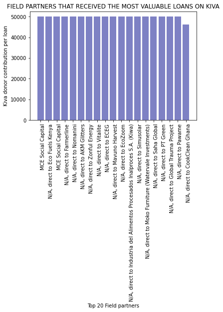
The per capita contribution shows most of the largest contributions per loan actually went directly to social impact businesses.

The characteristics of KIVA borrowers#

In this section, we seek to understand KIVA borrower characteristics.

1. What is the size of the shortfall for each individual borrower in a given sector?

# create a pivot-table
tab6 = pd.pivot_table(loan_data_copy, values='funded_amount', index=['sector'], aggfunc='sum')

# sort the results in descending order
tab6 = tab6.sort_values(by=['funded_amount'], ascending=False)

# rename the aggregated column to an appropiate label
tab6.columns = ['sum_of_funded_amount']

# make some index entries into columns
tab6 = tab6.reset_index(level=['sector'])

# create another pivot-table
loans_by_sector = pd.pivot_table(loan_data_copy, values='id', index=['sector'], aggfunc='count')

# sort the results in descending order
loans_by_sector = loans_by_sector.sort_values(by=['id'], ascending=False)

# rename the aggregated column to an appropiate label
loans_by_sector.columns = ['number_of_loans']

# make some index entries into columns
loans_by_sector = loans_by_sector.reset_index(level=['sector'])

# create a third pivot-table
loan_amounts_by_sector = pd.pivot_table(loan_data_copy, values='loan_amount', index=['sector'], aggfunc='sum')

# sort the results in descending order
loan_amounts_by_sector = loan_amounts_by_sector.sort_values(by=['loan_amount'], ascending=False)

# rename the aggregated column to an appropiate label
loan_amounts_by_sector.columns = ['sum_of_loan_amount']

# make some index entries into columns
loan_amounts_by_sector = loan_amounts_by_sector.reset_index(level=['sector'])

# initial status message
print('The shape of tab6 before merge: ', tab6.shape)

# join the data, keeping only relevant entries
tab6 = tab6.merge(loans_by_sector, on='sector')

# final status message
print('The shape of tab6 after merge: ', tab6.shape)


# initial status message
print('The shape of tab6 before merge: ', tab6.shape)

# join the data, keeping only relevant entries
tab6 = tab6.merge(loan_amounts_by_sector, on='sector')

# final status message
print('The shape of tab6 after merge: ', tab6.shape)

The shape of tab6 before merge:  (15, 2)
The shape of tab6 after merge:  (15, 3)
The shape of tab6 before merge:  (15, 3)
The shape of tab6 after merge:  (15, 4)

# assess additional metrics
tab6.loc[:, 'donor_contribution_per_loan'] = tab6['sum_of_funded_amount']/tab6['number_of_loans']
tab6.loc[:, 'funding_gap_per_loan'] = (-tab6['sum_of_loan_amount']+tab6['sum_of_funded_amount'])/tab6['number_of_loans']

# sort the results in descending order
tab6 = tab6.sort_values(by=['donor_contribution_per_loan'], ascending=False)

# display all results

fig, ax = plt.subplots()

ax.bar(tab6.iloc[:,0], tab6.iloc[:,4], color='#7e81c4')

plt.ylabel('Kiva donor contribution per loan')

ax.set_xticklabels(labels=tab6.iloc[:,0], rotation = (90), fontsize = 10, va='top', ha='left')

plt.xlabel('Sectors')

plt.title('SECTORS THAT RECEIVED THE MOST VALUABLE LOANS ON KIVA')

plt.show()

# sort the results in descending order
tab6 = tab6.sort_values(by=['funding_gap_per_loan'], ascending=False)

# display all results

fig, ax = plt.subplots()

ax.bar(tab6.iloc[:,0], tab6.iloc[:,5], color='crimson')

plt.ylabel('Funding gap per loan')

ax.set_xticklabels(labels=tab6.iloc[:,0], rotation = (90), fontsize = 10, va='top', ha='left')

plt.xlabel('Sectors')

plt.title('SECTORS THAT HAD THE LARGEST FUNDING GAP ON KIVA')

plt.show()

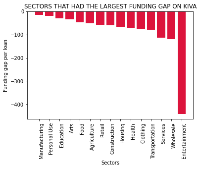
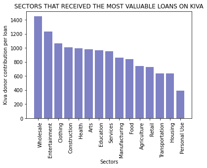
In as much as Entertainment has the second most valuable loans, it appears that this sector had the highest funding gap. Manufacturing had the lowest funding gap.

2. How were loans and funding distributed across the genders?

loan_data_copy.loc[:, 'number_of_all_borrowers'] = loan_data_copy['borrower_genders'].str.count('male') # counts both instances of female and male - they share the 'male' element
loan_data_copy.loc[:, 'number_of_female_borrowers'] = loan_data_copy['borrower_genders'].str.count('female')
loan_data_copy.loc[:, 'number_of_male_borrowers'] = loan_data_copy['number_of_all_borrowers'] - loan_data_copy['number_of_female_borrowers']


print('We had borrower data on',
      round(loan_data_copy['number_of_all_borrowers'].count()/loan_data_copy.shape[0]*100, 2),
      '% of the loans recorded')

We had borrower data on 99.37 % of the loans recorded

How different genders group together to borrow on Kiva

# create a pivot-table
borrower_group_data = pd.pivot_table(loan_data_copy, values=['number_of_male_borrowers', 'number_of_female_borrowers'],
                                     index=['number_of_all_borrowers'],aggfunc='sum')
#N/B: Using the count gives the total number of loans with borrower data; we need the sum to see the gender distribution across group size

# make some index entries into columns
borrower_group_data = borrower_group_data.reset_index(level=['number_of_all_borrowers'])


# display the results
fig, ax = plt.subplots()

ax.bar(borrower_group_data.iloc[:,0], borrower_group_data.iloc[:,2],
       label='Men', color='#7e81c4')

ax.bar(borrower_group_data.iloc[:,0], borrower_group_data.iloc[:,1],
       bottom=borrower_group_data.iloc[:,2], label='Women', color='#cbcce7')

ax.set_ylabel('Number of borrowers')

ax.set_xlabel('Size of borrower groups')

ax.set_title('GENDER AND SIZE OF BORROWER GROUPS')

ax.legend()

plt.show()

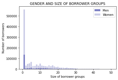
The graph above shows that most people preferred to borrow as individuals; however, there were substantially larger numbers of women in each group size compared to men.

Most common nationalities for the different genders

# create a pivot-table
borrower_country_data = pd.pivot_table(loan_data_copy, values=['number_of_male_borrowers', 'number_of_female_borrowers'],
                                       index=['country'],aggfunc='sum')


# sort the male results in descending order
borrower_country_data = borrower_country_data.sort_values(by=['number_of_male_borrowers'], ascending=False)

# make some index entries into columns
borrower_country_data = borrower_country_data.reset_index(level=['country'])


# display the results
fig, ax = plt.subplots()

ax.bar(borrower_country_data.iloc[0:10,0], borrower_country_data.iloc[0:10,2],
       label='Men', color='#7e81c4')

ax.bar(borrower_country_data.iloc[0:10,0], borrower_country_data.iloc[0:10,1],
       bottom=borrower_country_data.iloc[0:10,2], label='Women', color='#cbcce7')

ax.set_xticklabels(labels=borrower_country_data.iloc[0:10,0], rotation = (90), fontsize = 10, va='top', ha='left')

ax.set_ylabel('Number of borrowers')

ax.set_xlabel('Top 10 countries for men')

ax.set_title('NUMBER OF BORROWERS BY GENDER AND COUNTRY')

ax.legend()

plt.show()

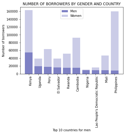
The country with the highest number of male borrowers was Kenya, while the country where men formed the majority of KIVA borrowers was Nigeria.

# sort the female results in descending order
borrower_country_data = borrower_country_data.sort_values(by=['number_of_female_borrowers'], ascending=False)

# display the results
fig, ax = plt.subplots()

ax.bar(borrower_country_data.iloc[0:10,0], borrower_country_data.iloc[0:10,2],
       label='Men', color='#7e81c4')

ax.bar(borrower_country_data.iloc[0:10,0], borrower_country_data.iloc[0:10,1],
       bottom=borrower_country_data.iloc[0:10,2], label='Women', color='#cbcce7')

ax.set_xticklabels(labels=borrower_country_data.iloc[0:10,0], rotation = (90),
                   fontsize = 10, va='top', ha='left')

ax.set_ylabel('Number of borrowers')

ax.set_xlabel('Top 10 countries for women')

ax.set_title('NUMBER OF BORROWERS BY GENDER AND COUNTRY')

ax.legend()

plt.show()

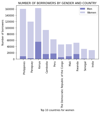
The country with the highest number of female borrowers was the Philippines, it can also be observed that nearly all borrowers were women in Paraguay and Senegal, while India appears to consist of only female borrowers.

# create a pivot-table
tab7 = pd.pivot_table(loan_data_copy, values=['term_in_months', 'number_of_all_borrowers', 'number_of_male_borrowers', 'number_of_female_borrowers', 'loan_amount', 'funded_amount'], index=['repayment_interval'], aggfunc='sum')

# sort the results in descending order
tab7 = tab7.sort_values(by=['number_of_all_borrowers'], ascending=False)

# make some index entries into columns
tab7 = tab7.reset_index(level=['repayment_interval'])

# create another pivot-table
loan_repayment = pd.pivot_table(loan_data_copy, values='id', index=['repayment_interval'], aggfunc='count')

# sort the results in descending order
loan_repayment = loan_repayment.sort_values(by=['id'], ascending=False)

# rename the aggregated column to an appropiate label
loan_repayment.columns = ['number_of_loans']

# make some index entries into columns
loan_repayment = loan_repayment.reset_index(level=['repayment_interval'])

# initial status message
print('The shape of tab7 before merge: ', tab7.shape)

# join the data, keeping only relevant entries
tab7 = tab7.merge(loan_repayment, on='repayment_interval')

# final status message
print('The shape of tab7 after merge: ', tab7.shape)

The shape of tab7 before merge:  (4, 7)
The shape of tab7 after merge:  (4, 8)

# Present findings in more digestible formats by:

# 1. Converting total borrowers to male and female proportions
tab7.loc[:, 'female_pct_of_total_borrowers'] = round((tab7['number_of_female_borrowers']/tab7['number_of_all_borrowers'])*100, 2)
tab7.loc[:, 'male_pct_of_total_borrowers'] = round((tab7['number_of_male_borrowers']/tab7['number_of_all_borrowers'])*100, 2)

# 2. Extracting funding amounts based on gender
tab7.loc[:, 'million_USD_female_total_funding'] = round((tab7['female_pct_of_total_borrowers']/100*tab7['funded_amount'])/1000000, 2)
tab7.loc[:, 'million_USD_male_total_funding'] = round((tab7['male_pct_of_total_borrowers']/100*tab7['funded_amount'])/1000000, 2)

# 3. Extracting loan amounts based on gender
tab7.loc[:, 'million_USD_female_total_loan_amount'] = round((tab7['female_pct_of_total_borrowers']/100*tab7['loan_amount'])/1000000, 2)
tab7.loc[:, 'million_USD_male_total_loan_amount'] = round((tab7['male_pct_of_total_borrowers']/100*tab7['loan_amount'])/1000000, 2)

# 4. Extracting funding gaps based on gender
tab7.loc[:, 'million_female_funding_gap'] = -tab7['million_USD_female_total_loan_amount']+tab7['million_USD_female_total_funding']
tab7.loc[:, 'million_male_funding_gap'] = -tab7['million_USD_male_total_loan_amount']+tab7['million_USD_male_total_funding']

# drop raw data columns
tab7 = tab7.drop(['funded_amount', 'loan_amount',
                  'number_of_all_borrowers', 'number_of_female_borrowers',
                  'number_of_male_borrowers'],1)

Funding received based on gender

# display summary of funding by gender

status = ['Total male funding','Total female funding']

values = [tab7['million_USD_male_total_funding'].sum(), tab7['million_USD_female_total_funding'].sum()]

fig1, ax1 = plt.subplots()

ax1.pie(values, labels=status,
        autopct='%1.2f%%',
        startangle=90,
        colors=np.array(['#7e81c4','#cbcce7']))

ax1.axis('equal')  # Equal aspect ratio ensures that pie is drawn as a circle.

plt.show()

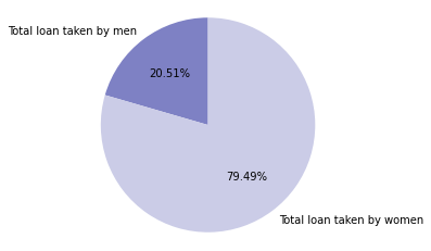
Total loan amounts taken by each gender

# display loan amounts by gender

status = ['Total loan taken by men','Total loan taken by women']

values = [tab7['million_USD_male_total_loan_amount'].sum(), tab7['million_USD_female_total_loan_amount'].sum()]

fig1, ax1 = plt.subplots()

ax1.pie(values, labels=status,
        autopct='%1.2f%%',
        startangle=90,
        colors=np.array(['#7e81c4','#cbcce7']))

ax1.axis('equal')  # Equal aspect ratio ensures that pie is drawn as a circle.

plt.show()

Loan repayment behaviour based on gender

# Display summary of loan repayment behaviour by gender
# 1. Men
fig, ax = plt.subplots()

ax.bar(tab7.iloc[:,0],
       (tab7.iloc[:,1]/tab7.iloc[:,2])*(tab7.iloc[:,4]/100),
       label='Men', color='#7e81c4')

ax.set_ylabel('Loan term per loan')

ax.set_xlabel('Repayment interval')

ax.set_title('LOAN REPAYMENT BEHAVIOUR')

ax.legend()

plt.show()

# 2. Women
fig, ax = plt.subplots()

ax.bar(tab7.iloc[:,0],
       (tab7.iloc[:,1]/tab7.iloc[:,2])*(tab7.iloc[:,3]/100),
       label='Women', color='#cbcce7')

ax.set_ylabel('Loan term per loan')

ax.set_xlabel('Repayment interval')

ax.set_title('LOAN REPAYMENT BEHAVIOUR')

ax.legend()

plt.show()

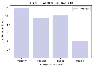
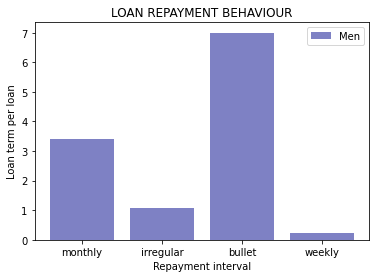
In as much as most men and women consistently paid off long-term loans on a monthly basis, women had a much larger time horizon to pay off their loans in general.

Additionally, a significant amount of data on repayment behaviour is missing for both genders (missing data is represented as the ‘bullet group’).

Funding gap in millions faced by each gender

# display summary of funding gap by gender

status = ['Male funding gap','Female funding gap']

values = [abs(tab7['million_male_funding_gap'].sum()), abs(tab7['million_male_funding_gap'].sum())]

fig1, ax1 = plt.subplots()

ax1.pie(values, labels=status,
        autopct='%1.2f%%',
        startangle=90,
        colors=np.array(['#7e81c4','#cbcce7']))

ax1.axis('equal')  # Equal aspect ratio ensures that pie is drawn as a circle.

plt.show()

print('In this instance, both men and women have the same size of funding gap, {} million US dollars\nover the time period the data was collected.'
      .format(round(
          abs(tab7['million_male_funding_gap'].sum()),
          2)
             )
     )

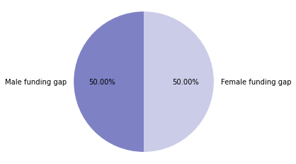
In this instance, both men and women have the same size of funding gap, 10.19 million US dollars
over the time period the data was collected.

# display summary of the funding gap by gender and monthly repayment behaviour
fig, ax = plt.subplots()

ax.bar(tab7.iloc[:,0], tab7.iloc[:,10], label='Men', color='black')

ax.bar(tab7.iloc[:,0], tab7.iloc[:,9], bottom=tab7.iloc[:,10], label='Women', color='crimson')

ax.set_ylabel('Funding gap (millions)')

ax.set_xlabel('Repayment interval')

ax.set_title('SIZE OF FUNDING GAP')

ax.legend()

plt.show()

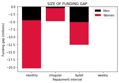
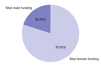
The graph above indicates that in as much as women are getting much more funding than men, those in the monthly repayment group still have a significant funding gap. Furthermore, the second-largest funding gap was not from those people belonging to the irregular payments group, but those belonging to the group that had missing data on payment behaviour. This makes sense because there may be a lack of trust that makes KIVA donors not foot the entire loan of those with missing repayment plans.

Global welfare#

In this section, we seek to explore the data to understand the financial well-being of various countries with the aid of an external dataset

1. What percentage of their monthly expenditure does the average citizen devote to loan repayments?

The purchasing power of various countries of the world can be visualized in the form of the monthly income table below:

# Made a copy of the data: 
expenditure = PCE_data.copy()

# Convert any 'n/a' strings to NaN values
expenditure = expenditure.replace('n/a', np.nan)

# Convert any numeric data stored as a string into a decimal
cols = expenditure.columns[1:61]

for col in cols:
    expenditure.loc[:,col] = expenditure[col].str.replace(',','')

for col in cols:
    expenditure.loc[:,col] = expenditure[col].astype('float64')
    
MonthlyExpenditure = (expenditure.loc[:,'2013':'2017'].copy())/12

MonthlyExpenditure.loc[:,'country'] = expenditure['Country']

# Drop any null columns
MonthlyExpenditure = MonthlyExpenditure.dropna()

MonthlyExpenditure

	2013	2014	2015	2016	2017	country
1	582.357500	586.271667	584.475000	591.529167	592.816667	American Samoa
2	61.932500	63.661667	66.361667	69.737500	71.814167	Cambodia
3	175.452500	190.616667	206.155833	223.367500	243.301667	China
5	164.263333	170.690000	176.700000	183.363333	190.249167	Indonesia
6	121.336667	124.944167	137.075833	141.720833	145.214167	Kiribati
...	...	...	...	...	...	...
179	91.753333	91.670000	92.621667	93.139167	93.662500	Sudan
180	42.089167	42.224167	43.976667	43.604167	43.282500	Tanzania
181	36.333333	37.132500	37.786667	38.175000	37.630833	Togo
182	54.592500	54.118333	57.973333	56.637500	54.675000	Uganda
184	84.350833	80.766667	94.590000	83.371667	83.315833	Zimbabwe

156 rows × 6 columns

In turn, the monthly repayments of various countries of the world can be visualized in the form of the monthly repayments table below:

# get the monthly repayment on each loan
loan_data_copy.loc[:, 'monthly_loan_repayment'] = loan_data_copy['loan_amount']/loan_data_copy['term_in_months']

# get the year that the loan was issued
loan_data_copy.loc[:,'disbursement_year'] = loan_data['disbursed_time'].dt.year

# create a pivot-table
tab8 = pd.pivot_table(loan_data_copy, values=['monthly_loan_repayment'], columns='disbursement_year', index=['country'], aggfunc='mean')

# drop level and rename columns
tab8 = tab8.droplevel('disbursement_year', axis=1)
tab8.columns = ['monthly_loan_repayment 2013', 'monthly_loan_repayment 2014',
                'monthly_loan_repayment 2015', 'monthly_loan_repayment 2016',
                'monthly_loan_repayment 2017']

# make some index entries into columns
tab8 = tab8.reset_index(level=['country'])

# and display all results
tab8

	country	monthly_loan_repayment 2013	monthly_loan_repayment 2014	monthly_loan_repayment 2015	monthly_loan_repayment 2016	monthly_loan_repayment 2017
0	Afghanistan	NaN	NaN	750.000000	1333.333333	NaN
1	Albania	62.227835	64.557728	54.131447	55.527071	61.604227
2	Armenia	64.103653	64.558263	51.850628	49.406712	50.580462
3	Azerbaijan	105.071779	108.725509	82.548595	59.692751	NaN
4	Belize	NaN	18.405275	NaN	22.880435	NaN
...	...	...	...	...	...	...
80	Vanuatu	NaN	62.500000	NaN	NaN	NaN
81	Vietnam	68.839701	91.272779	97.516549	90.730029	69.997056
82	Yemen	62.567830	57.303204	60.290609	43.056244	42.720586
83	Zambia	NaN	81.800068	93.311061	107.013918	74.278048
84	Zimbabwe	175.857143	74.398992	126.842706	110.083632	125.510372

85 rows × 6 columns

We need to find the countries shared in common between the Kiva.org and the UN dataset as follows:

# compare country/territory labels in the 2 datasets
print(tab8['country'].unique())
print('')
print(MonthlyExpenditure['country'].unique())

['Afghanistan' 'Albania' 'Armenia' 'Azerbaijan' 'Belize' 'Benin' 'Bhutan'
 'Bolivia' 'Brazil' 'Burkina Faso' 'Burundi' 'Cambodia' 'Cameroon' 'Chile'
 'China' 'Colombia' 'Congo' 'Costa Rica' "Cote D'Ivoire"
 'Dominican Republic' 'Ecuador' 'Egypt' 'El Salvador' 'Georgia' 'Ghana'
 'Guatemala' 'Haiti' 'Honduras' 'India' 'Indonesia' 'Iraq' 'Israel'
 'Jordan' 'Kenya' 'Kosovo' 'Kyrgyzstan' "Lao People's Democratic Republic"
 'Lebanon' 'Lesotho' 'Liberia' 'Madagascar' 'Malawi' 'Mali' 'Mauritania'
 'Mexico' 'Moldova' 'Mongolia' 'Mozambique' 'Myanmar (Burma)' 'Namibia'
 'Nepal' 'Nicaragua' 'Nigeria' 'Pakistan' 'Palestine' 'Panama' 'Paraguay'
 'Peru' 'Philippines' 'Puerto Rico' 'Rwanda'
 'Saint Vincent and the Grenadines' 'Samoa' 'Senegal' 'Sierra Leone'
 'Solomon Islands' 'Somalia' 'South Africa' 'South Sudan' 'Suriname'
 'Tajikistan' 'Tanzania' 'Thailand' 'The Democratic Republic of the Congo'
 'Timor-Leste' 'Togo' 'Turkey' 'Uganda' 'Ukraine' 'United States'
 'Vanuatu' 'Vietnam' 'Yemen' 'Zambia' 'Zimbabwe']

['American Samoa' 'Cambodia' 'China' 'Indonesia' 'Kiribati' 'Malaysia'
 'Marshall Islands' 'Mongolia' 'Northern Mariana Islands' 'Palau'
 'Philippines' 'Thailand' 'Timor-Leste' 'Vietnam' 'Albania' 'Armenia'
 'Belarus' 'Bosnia and Herzegovina' 'Bulgaria' 'Croatia' 'Czech Republic'
 'Estonia' 'Georgia' 'Hungary' 'Kazakhstan' 'Kosovo' 'Kyrgyz Republic'
 'Latvia' 'Lithuania' 'Moldova' 'Montenegro' 'North Macedonia' 'Poland'
 'Romania' 'Russian Federation' 'Serbia' 'Slovak Republic' 'Slovenia'
 'Turkey' 'Ukraine' 'Uzbekistan' 'Argentina' 'Belize' 'Bolivia' 'Brazil'
 'Chile' 'Colombia' 'Costa Rica' 'Cuba' 'Dominican Republic' 'Ecuador'
 'El Salvador' 'Guatemala' 'Haiti' 'Honduras' 'Jamaica' 'Mexico'
 'Nicaragua' 'Panama' 'Paraguay' 'Peru' 'Uruguay' 'Algeria'
 'Egypt, Arab Republic of' 'Iran, Islamic Republic of' 'Jordan' 'Lebanon'
 'Morocco' 'Oman' 'West Bank and Gaza' 'Australia' 'Austria'
 'Bahamas, The' 'Bahrain' 'Belgium' 'Brunei Darussalam' 'Canada' 'Cyprus'
 'Denmark' 'Finland' 'France' 'Germany' 'Greece' 'Greenland' 'Guam'
 'Hong Kong SAR, China' 'Iceland' 'Ireland' 'Israel' 'Italy' 'Japan'
 'Korea, Republic of' 'Kuwait' 'Luxembourg' 'Macao SAR, China'
 'Netherlands' 'New Zealand' 'Norway' 'Portugal' 'Puerto Rico'
 'Saudi Arabia' 'Singapore' 'Spain' 'Sweden' 'Switzerland'
 'United Arab Emirates' 'United Kingdom' 'United States'
 'Virgin Islands, US' 'Bangladesh' 'Bhutan' 'India' 'Nepal' 'Pakistan'
 'Sri Lanka' 'Angola' 'Benin' 'Botswana' 'Burkina Faso' 'Burundi'
 'Cabo Verde' 'Cameroon' 'Central African Republic' 'Chad' 'Comoros'
 'Congo, Democratic Republic of' 'Congo, Republic of' "Cote d'Ivoire"
 'Equatorial Guinea' 'Eswatini' 'Gabon' 'Gambia, The' 'Ghana' 'Guinea'
 'Guinea-Bissau' 'Kenya' 'Lesotho' 'Liberia' 'Madagascar' 'Malawi' 'Mali'
 'Mauritania' 'Mauritius' 'Mozambique' 'Namibia' 'Niger' 'Nigeria'
 'Rwanda' 'Senegal' 'Sierra Leone' 'South Africa' 'Sudan' 'Tanzania'
 'Togo' 'Uganda' 'Zimbabwe']

# MATCH COUNTRIES IN KIVA LOAN DATA AND THOSE IN THE ORIGINAL DATASET IF THEY HAVE DIFFERENT SPELLINGS 

tab8.iloc[16,0] = 'Congo, Republic of'
tab8.iloc[18,0] = "Cote d'Ivoire"
tab8.iloc[21,0] = 'Egypt, Arab Republic of'
tab8.iloc[35,0] = 'Kyrgyz Republic'
tab8.iloc[48,0] = 'Myanmar'
tab8.iloc[54,0] = 'West Bank and Gaza'
# tab8.iloc[61,0] missing in other dataset
# tab8.iloc[62,0] missing in other dataset; only have American Samoa

# tab8.iloc[63,0] missing in other dataset
# tab8.iloc[65,0] missing in other dataset
# tab8.iloc[66,0] missing in other dataset
tab8.iloc[73,0] = 'Congo, Democratic Republic of'
# tab8.iloc[82,0] missing in other dataset

#CHECK FOR COUNTRIES NOT WITHIN EITHER ONE OF THE DATASET
tab8[tab8['country'].isin(MonthlyExpenditure['country']) == False]

	country	monthly_loan_repayment 2013	monthly_loan_repayment 2014	monthly_loan_repayment 2015	monthly_loan_repayment 2016	monthly_loan_repayment 2017
0	Afghanistan	NaN	NaN	750.000000	1333.333333	NaN
3	Azerbaijan	105.071779	108.725509	82.548595	59.692751	NaN
30	Iraq	173.604827	198.899334	186.551621	NaN	NaN
36	Lao People's Democratic Republic	NaN	122.887368	76.689249	78.100108	55.966610
48	Myanmar	NaN	1084.647495	301.828805	153.652721	80.601104
61	Saint Vincent and the Grenadines	NaN	43.601190	91.355946	NaN	NaN
62	Samoa	45.125878	64.451621	56.148887	63.796669	60.880531
65	Solomon Islands	NaN	50.795455	64.064459	79.784429	69.712160
66	Somalia	NaN	272.774699	230.544232	564.285714	510.714286
68	South Sudan	NaN	75.533234	44.681710	NaN	6250.000000
69	Suriname	NaN	331.387203	232.768221	263.640545	NaN
70	Tajikistan	67.230372	66.099868	53.060960	40.184397	37.572885
80	Vanuatu	NaN	62.500000	NaN	NaN	NaN
82	Yemen	62.567830	57.303204	60.290609	43.056244	42.720586
83	Zambia	NaN	81.800068	93.311061	107.013918	74.278048

The table above shows countries that are missing in either of the datasets and will not be included.

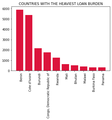
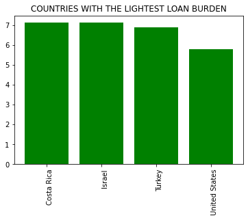
The percentage of monthly expenditure that the average citizen devote to loan repayments is visualized below:

# initial status message
print('The shape of tab8 before merge: ', tab8.shape)

# join the data, keeping only relevant entries
tab8 = tab8.merge(MonthlyExpenditure, on='country')

# final status message
print('The shape of tab8 after merge: ', tab8.shape)

The shape of tab8 before merge:  (85, 6)
The shape of tab8 after merge:  (70, 11)

years = ['2013','2014','2015','2016','2017']

for year in years:
    tab8.loc[:, f'% of monthly expenditure, {year}'] = (tab8[f'monthly_loan_repayment {year}']/tab8[f'{year}']) * 100
    tab8[f'% of monthly expenditure, {year}'] = round(tab8[f'% of monthly expenditure, {year}'], 2)
    tab8 = tab8.drop([f'monthly_loan_repayment {year}',f'{year}'], axis=1)

# sort the results in descending order
tab8 = tab8.sort_values(by=['% of monthly expenditure, 2017'], ascending=False)

fig, ax = plt.subplots()

ax.bar(tab8.head(10).iloc[:,0],
       tab8.head(10)['% of monthly expenditure, 2017'],
       color='crimson')

#plt.ylabel('Funding gap per loan')

ax.set_xticklabels(labels=tab8.head(10).iloc[:,0], rotation = (90), fontsize = 10, va='top', ha='left')

#plt.xlabel('Sectors')

plt.title('COUNTRIES WITH THE HEAVIEST LOAN BURDEN')

plt.show()

print ('\n')

fig, ax = plt.subplots()

ax.bar(tab8.tail(10).iloc[:,0],
       tab8.tail(10)['% of monthly expenditure, 2017'],
       color='green')

#plt.ylabel('Funding gap per loan')

ax.set_xticklabels(labels=tab8.tail(10).iloc[:,0], rotation = (90), fontsize = 10, va='top', ha='left')

#plt.xlabel('Sectors')

plt.title('COUNTRIES WITH THE LIGHTEST LOAN BURDEN')

plt.show()

2. What geographical regions have the highest and lowest levels of poverty?

This is measured by the Multidimensional Poverty Index (MPI). This was obtained as follows:

print(loan_data_copy.shape)
print('Number of null values in the "region" column: ',loan_data_copy['region'].isnull().sum())
print('Number of null values in the "country_code" column: ',loan_data_copy['country_code'].isnull().sum())
print('Number of null values in the "country" column: ',loan_data_copy['country'].isnull().sum())
print('')
print('N/B: ', loan_data_copy[loan_data_copy['region'].isin(location_data['region']) == False].shape[0],
      'number of loan records have regions that are not covered in both datasets.')
print('     ', loan_data_copy[loan_data_copy['country'].isin(location_data['country']) == False].shape[0],
      'number of loan records have countries that are not covered in both datasets.')

(671205, 26)
Number of null values in the "region" column:  56800
Number of null values in the "country_code" column:  8

Number of null values in the "country" column:  0

N/B:  558379 number of loan records have regions that are not covered in both datasets.

      80765 number of loan records have countries that are not covered in both datasets.

Based on country:

# Let's first get a national average for MPI
# create a pivot-table
tab9 = pd.pivot_table(location_data, values=['MPI'], index=['country'], aggfunc='min')

# rename the MPI
tab9.columns = ['national_minimum_of_MPI']

# make some index entries into columns
tab9 = tab9.reset_index(level=['country'])

# sort the results in descending order
tab9 = tab9.sort_values(by=['national_minimum_of_MPI'], ascending=False)

# display all results
fig, ax = plt.subplots()
ax.bar(tab9.iloc[0:10,0], tab9.iloc[0:10,1], color='crimson')
plt.ylabel('MPI (national minimum)')
ax.set_xticklabels(labels=tab9.iloc[0:10,0], rotation = (90), fontsize = 10, va='top', ha='left')
plt.xlabel('Top 10 countries')
plt.title('COUNTRIES THAT HAD THE HIGHEST LEVEL OF POVERTY AS AT 2017')
plt.show()

print('\n')

# sort the results in ascending order
tab9 = tab9.sort_values(by=['national_minimum_of_MPI'], ascending=True)

# display all results
fig, ax = plt.subplots()
ax.bar(tab9.iloc[0:10,0], tab9.iloc[0:10,1], color='green')
plt.ylabel('MPI (national minimum)')
ax.set_xticklabels(labels=tab9.iloc[0:10,0], rotation = (90), fontsize = 10, va='top', ha='left')
plt.xlabel('Bottom 10 countries')
plt.title('COUNTRIES THAT HAD THE LOWEST LEVEL OF POVERTY AS AT 2017')
plt.show()

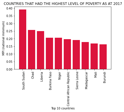
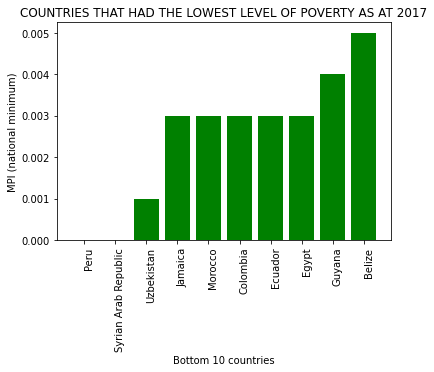
Based on the results above, countries with high MPI values are not receiving the most funding - in fact, El-Salvador, a country with one of the lowest MPI scores was one of the top 10 countries that received the most funding.

Based on in-country regions:

region_data = loan_data_copy[loan_data_copy['region'].isin(location_data['region']) == True]
region_data = region_data.copy()

tab10 = pd.pivot_table(region_data, values=['funded_amount', 'loan_amount',
                                            'number_of_all_borrowers', 'monthly_loan_repayment'],
                       index=['region'], aggfunc='sum')

# make some index entries into columns
tab10 = tab10.reset_index(level=['region'])

tab11 = pd.pivot_table(region_data, values=['id'],
                       index=['region'], aggfunc='count')

# rename the aggregated column
tab11.columns = ['number_of_loans']

# make some index entries into columns
tab11 = tab11.reset_index(level=['region'])

# initial status message
print('The shape of tab10 before merge: ', tab10.shape)

# join the data, keeping only relevant entries
tab10 = tab10.merge(tab11, on='region')

# final status message
print('The shape of tab10 after merge: ', tab10.shape)


# initial status message
print('The shape of tab10 before merge: ', tab10.shape)

# join the data, keeping only relevant entries
tab10 = tab10.merge(location_data, on='region')

# final status message
print('The shape of tab10 after merge: ', tab10.shape)

The shape of tab10 before merge:  (131, 5)
The shape of tab10 after merge:  (131, 6)
The shape of tab10 before merge:  (131, 6)
The shape of tab10 after merge:  (144, 14)

# sort the results in descending order
tab10 = tab10.sort_values(by=['MPI'], ascending=False)

# display all results
fig, ax = plt.subplots()
ax.bar(tab10.iloc[0:10,6], tab10.iloc[0:10,10], color='crimson')
plt.ylabel('MPI')
ax.set_xticklabels(labels=tab10.iloc[0:10,6], rotation = (90), fontsize = 10, va='top', ha='left')
plt.xlabel('Top 10 regions')
plt.title('REGIONS THAT HAD THE HIGHEST LEVEL OF POVERTY AS AT 2017')
plt.show()

print('\n')

# sort the results in ascending order
tab10 = tab10.sort_values(by=['MPI'], ascending=True)

# display all results
fig, ax = plt.subplots()
ax.bar(tab10.iloc[0:10,6], tab10.iloc[0:10,10], color='green')
plt.ylabel('MPI')
ax.set_xticklabels(labels=tab10.iloc[0:10,6], rotation = (90), fontsize = 10, va='top', ha='left')
plt.xlabel('Bottom 10 regions')
plt.title('REGIONS THAT HAD THE LOWEST LEVEL OF POVERTY AS AT 2017')
plt.show()

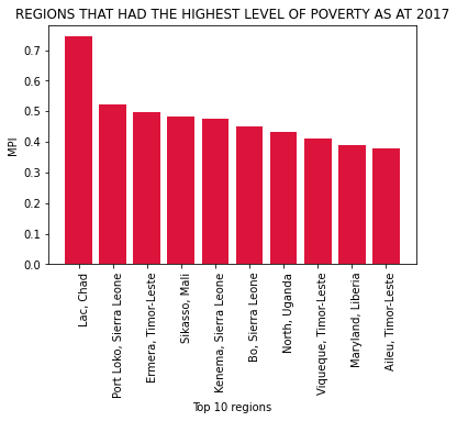
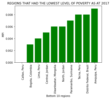
Peru has the third highest number of loans and it is the third most funded country; based on the graph above, it has 3 regions among countries with the lowest MPI scores with the fourth region having an unknown MPI score.

Conclusions#

The welfare of borrowers that receive the largest amount of funding on Kiva can be viewed as good because:

Women form the bulk of the borrowers and they receive the highest number of funds, even as they have the highest shortfall.
Countries like Peru and El Salvador which based on the data have low MPI scores have received a lot of funding
The most valuable partnerships are those with social impact businesses, which implies that they are able to hanle regular payments as they make an income from their goods and services
Few borrowers are taking loans for personal use
Kenya and the Phillipines have a lot of funding for small loans; this implies that massive impact is being achieved in these countries because the loans are small enough to pay back and monthly repayments are taking up only 50% or less of their monthly income

With that said, it is concerning to see that countries that have many more people in need are not accessing large amounts of funds; furthermore, even when they do, places like Burkina Faso, Sierra Leone and Mali had a high debt burden, trapping borrowers from these countries in poverty.

My Knowledge Hub

Kiva Project

Contents